Author Archive

Suburban Nation: U.S. 86 Percent Suburban

From Jurisdictional to Functional Analysis of Urban Cores & Suburbs

For decades there has been considerable analysis of urban core versus suburban trends. However, for the most part, analysts have been jurisdictional, comparing historical core municipalities to the expanse that constitutes the rest of the metropolitan area. Most core municipalities are themselves substantially suburban, which can mask (and exaggerate) the size of urban cores and understate the extent of suburbanization.

Our new City Sector Model evaluates the more than 8,900 zip codes in the 52 U.S. metropolitan areas that have more than 1,000,000 residents (“major metropolitan areas”) based on travel behavior and urban form. There are four categories, including  (1) Pre-Auto Urban Core, (2) Auto Suburban: Earlier, (3) Auto Suburban: Later and (4) Auto Exurban. It is recognized that automobile oriented suburbanization was underway before World War II, but it was interrupted by the Great Depression during the 1930s and was small compared to the democratization of personal mobility and home ownership that has occurred since that time.

Canada: A Suburban Nation

The City Sector Model is broadly similar to the groundbreaking research published by David L. A. Gordon and Mark Janzen at Queen’s University in Kingston Ontario (Suburban Nation: Estimating the Size of Canada’s Suburban Population) on the metropolitan areas of Canada. Gordon and Janzen concluded that the metropolitan areas of Canada are largely suburban. Among the major metropolitan areas of Canada, the Auto Suburbs and Exurbs combined contain 76 percent of the population, somewhat less than the 86 percent in the United States.

All U.S. Major Metropolitan Area Growth Has Been Suburban and Exurban

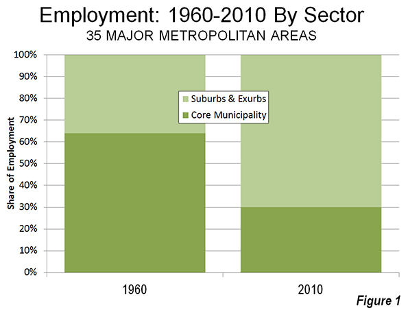
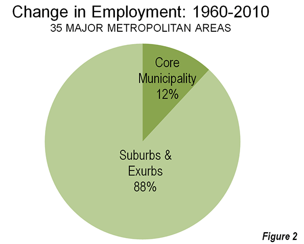
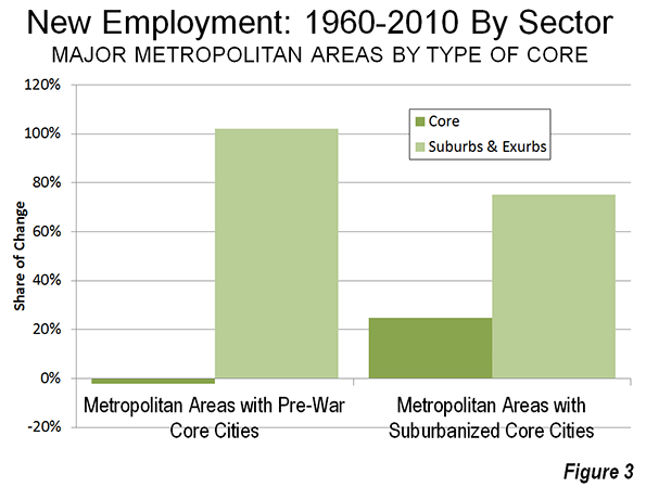
Virtually all population growth in U.S. metropolitan areas (as currently defined) has been suburban or exurban since before World War II (the 1940 census). The historical core municipalities that have not annexed materially and were largely developed by 1940 have lost population. Approximately 110 percent of their metropolitan area growth has occurred in suburbs and exurbs. Further, among the other core municipalities, virtually all of the population growth that has occurred in annexed areas or greenfield areas since 1940.

Identifying the Pre-Auto Urban Core

Not being constrained by municipal boundaries is important because core municipalities vary substantially. For example, the core municipality represents less than 10 percent of the population of Atlanta, while the core municipality represents more than 60 percent of the population of San Antonio. The City Sector Model applies data available from the U.S. Census Bureau to estimate the population and distribution of Pre-Auto Urban Cores in a consistent manner.

At the same time, the functional analysis is materially different from the Office of Management and Budget (OMB) classification of “principal cities.” It also differs from the Brookings Institution “primary cities,” which is based on the OMB approach. The OMB based classifications classify municipalities using employment data, without regard to urban form, density or other variables that are associated with the urban core. These classifications are useful and acknowledge that the monocentric nature of US metropolitan areas has evolved to polycentricity. However, non-urban core principal cities and primary cities are themselves, with few exceptions, functionally suburban (some of the most significant examples are Mesa, Arizona in the Phoenix area, which had a population of only 7,000 in 1940 and Arlington, Texas, in the Dallas-Fort Worth area, which had a population of only 4,000. Their populations, now both 350,000 or more are virtually all automobile oriented suburban).

The City Sector Model Criteria

Because of the substantial interest of urban planners in minimizing the use of automobiles and restoring transit, walking and cycling as primary urban travel alternatives, it is important to identify the extent of automobile oriented suburbanization to the greatest extent possible. Better information is required, regardless of an analysts’ orientation. (As an aside, this author believes that the data shows planning efforts to lead to lower standards of living and greater poverty, which is discussed in Toward More Prosperous Cities).

A number of data combinations were tested for the Pre-Auto Urban Core, to replicate as closely as feasible the 2010 population of the core municipalities that have virtually the same boundaries as in 1940 and that were virtually fully developed by that time (the Pre-War & Non-Suburban classification in historical core municipalities). The following criteria were accepted (represented graphically).

  •  The Auto Exurban category includes any area outside a principal urban area.
  •  The Pre-Auto Urban Core category includes any non-exurban with a median house construction date of 1945 or before and also included areas with a population density of 7,500 per square mile (2,900) or more and with a transit, walk and cycling journey to work market share of 20 percent or more.
  •  The Auto Suburban Earlier category included the balance of areas with a median house construction date of 1979 or before.
  •  The Auto Suburban Later category later included the balance of areas with a median house construction date of 1980 or later.

Additional details on the criteria are in the Note.

Results: 2010 Census

 The combined Pre-Auto Urban Core areas represented 14.4 percent of the population of the major metropolitan areas in 2010 (2013 geographical definition). This compares to the 26.4 percent that the core municipalities themselves represented of the metropolitan areas, indicating their large functionally suburban components.

The Auto Suburban: Earlier areas accounted for 42.0 percent of the population, while the Auto Suburban: Later areas had 26.8 percent of the population. The Auto Exurban areas had 16.8 percent of the population.

The substantial difference between U.S. and Canadian urbanization is illustrated by applying an approximation of the Gordon-Janzen criteria, which yielded an 8.4 percent Pre-Auto Urban Core population. The corresponding figure for the six major metropolitan areas of Canada was 24.0 percent. This difference is not surprising, since major Canadian urban areas have generally higher densities and much more robust transit, walking and cycling market shares. Yet, the Gordon-Janzen research shows Canada to be overwhelmingly suburban.

Population Density: As would be expected, the Pre-Auto Urban Core areas had the highest densities, at 11,000 per square mile (4,250 per square kilometer). The Auto Suburban: Earlier areas had a density of 2,500 per square mile (1,000 per square kilometer), while the Auto Suburban: Later had a population density of 1,300 per square mile (500 per square kilometer), while the Auto Exurban areas had a population density of 150 per square mile (60 per square kilometer).

Individual Metropolitan Areas (Cities)

The metropolitan areas with the highest proportion of Pre-Auto Urban Core population are New York (more than 50 percent), and Boston (nearly 35 percent), followed by Buffalo, Chicago, San Francisco-Oakland and Providence, all with more than 25 percent.

It may be surprising that many of the major metropolitan areas are shown with little or no Pre-Auto Urban Core population. For example, five metropolitan areas have no Pre-Auto Urban Core population, including Phoenix, Riverside-San Bernardino, Tampa-St. Petersburg, Orlando, Jacksonville and Birmingham. By the Census Bureau criteria of 1940, two of these areas were not yet metropolitan and only Birmingham (400,000) had more than 250,000 residents. Only the larger metropolitan had strong Pre-Auto Urban Cores. Many of the newer and fastest growing metropolitan areas were too small, too sparsely settled or insufficiently dense to have had strong urban cores before the great automobile suburbanization that followed World War II. Further, many of the Pre-Auto Urban Cores have experienced significant population loss and some of their neighborhoods have become more suburban (automobile oriented). Virtually no urban cores have been developed since World War II meeting the criteria.

Thus, no part of Phoenix, San Jose, Charlotte and a host of other newer metropolitan areas functionally resembles the Pre-Auto Urban Core areas of metropolitan areas like Chicago, Cincinnati or Milwaukee. However, new or expanded urban cores are possible, if built at high enough population density and with high enough transit, walking and cycling use.

Despite the comparatively small share of the modern metropolitan area represented by the Pre-Auto Urban Core in the City Core Model, the definition is broad and, if anything over-estimates the size of urban core city sectors. The population density of Pre-Auto Urban Core areas is below that of the historical core municipalities before the great auto oriented urbanization (11,000 compared to 12,100 in 1940) and well above their 2010 density (8,400), even when New York is excluded. The minimum density requirement of 7,500 per square mile (not applied to analysis zones with a median house construction data of 1945 or earlier) is slightly less than the density of Paris suburbs (7,800 per square mile or 3,000 per square kilometer) and only 20 percent more dense than the jurisdictional suburbs of Los Angeles (6,400 per square mile or 2,500 per square kilometer). Some urban containment plans require higher minimum densities, not only in urban cores but also in the suburbs.

The United States: An Even More Suburban Nation

In describing the Canadian results, Professor Gordon noted that there is a tendency to “overestimate the importance of the highly visible downtown cores and underestimate the vast growth happening in the suburban edges.” That is true to an even greater degree in the United States.

—–

Note: The City Sector Model is applied to the 52 major metropolitan areas in the United States (over 1 million population). The metropolitan areas are divided into the principal urban areas, with areas outside categorized as exurban. The principal urban areas in Los Angeles and San Francisco encompass the smaller Mission Viejo and Concord urban areas, which are adjacent. As a result, some smaller urban areas, such as Palm Springs (Riverside-San Bernardino metropolitan area), Lancaster (Los Angeles metropolitan area) and Poughkeepsie (New York metropolitan area) are considered exurban. Areas with less than 250 residents per square mile (100 per square kilometer) are also considered exurban, principally for classification of large areas on the urban fringe that have a substantial rural element.

The Pre-Auto Urban Core includes all non -– exurban areas in which is the house construction date is 1945 or before. In addition, the urban core includes areas that have a population density of 7,500 per square mile (2,900 per square kilometer) or more and a transit, walking and cycling journey to work market share of 20 percent or more, so long as they are in the urban area.

The analysis zones (zip codes) have an average population of 19,000, with from as many as 1,000 zones in New York to 50 in Raleigh.

—–

This article is adapted from From Jurisdictional to Functional Analysis of Urban Cores and Suburbs, originally published in newgeography.com. That article contains charts, tables and representative maps.

Smart Growth: Destroying Housing Opportunity from California to Australia (and Beyond)

Two recent stories provide further  evidence on the extent to which urban containment policies (also called smart growth, growth management, compact city policy, livability and urban consolidation) raises house prices relative to incomes, thereby reducing housing affordability. Because housing represents the largest element of household budgets (not transportation as a US government website implies), urban containment policy reduces discretionary income — the money households have left over after taxes and paying for necessities. This leads to a lower standard of living and more poverty, and violates the fundamental purposes of urban planning, described by former World Bank principal planner Alain Bertaud as:

“Increasing mobility and affordability are the two main objectives of urban planning. These two objectives are directly related to the overall goal of maximizing the size of a city’s labor market, and therefore, its economic prosperity.”

Two recent stories describe the effects of urban containment policy on the standard of living:

The Economist and Urban Containment “Fat Cats”

“Free Exchange” in The Economist came  down strongly on the side of economics in a review of housing affordability.

According to The Economist, the unusually high cost of housing in San Francisco (and other places) is principally the result of tight land use regulation, which makes it expensive or impossible to build. If “local regulations did not do much to discourage creation of new housing supply, then the market for San Francisco would be pretty competitive.” Add to that Vancouver, Sydney, Melbourne, Toronto, Portland and a host of additional metropolitan areas, where urban containment policy has driven house prices well above the 3.0 median multiple indicated by historic market fundamentals.

The Economist explains the issue in greater detail: “We therefore get highly restrictive building regulations. Tight supply limits mean that the gap between the marginal cost of a unit of San Francisco and the value to the marginal resident of San Francisco (and the market price of the unit) is enormous. That difference is pocketed by the rent-seeking NIMBYs of San Francisco. However altruistic they perceive their mission to be, the result is similar to what you’d get if fat cat industrialists lobbied the government to drive their competition out of business.” (Our emphasis).

Of course urban planning interests have long denied that that rationing land is associated with higher housing prices (read greater poverty and a lower standard of living). Nonetheless urban containment policies not only drive up the price of land, but do so even as they reduce the amount of land used for each new residence, driving prices per square foot of land up as well.

The Economist notes that unless the direction is changed, housing policy will continue to be “an instrument of oligarchy. Who knows. But however one imagines this playing out, we should be clear about what is happening, and what its effects have been.”

Land Prices Skyrocket as Residential Lot Sizes Fall in Australia

The extent to which smart growth policy (urban continament policy or urban consolidation policy) is associated with higher land (and house) prices is illustrated by a recent press release from RP Data in Australia. The analysis examined the vacant building lot prices for the period of 1993 to 2013.

During the period, the median price of a vacant lot rose 168 percent after adjustment for inflation.This is nearly 5 times the increase in the median household incomes of the seven largest capital cities (Sydney, Melbourne, Brisbane, Perth, Adelaide, Canberra and Sydney).

But it gets worse. The median lot size was reduced nearly 30 percent. This should put paid to the myth that urban containment reduces lot prices as it reduces their sizes. The same dynamic has been indicated in the United States.

Australia has been plagued by huge house cost increases relative to incomes in association with urban containment policy. Before the adoption of urban containment policy, it was typical for house prices to average three times or less than that of household income. Now, Sydney has the highest median multiple (median house price divided by median household income) of any major metropolitan area in the New World, with the exceptions of Vancouver and San Francisco. Melbourne, the second largest metropolitan area in Australia, has a median multiple of 8.4, making it fifth most costly in the New World, behind San Jose. All of Australia’s major metropolitan areas are “severely unaffordable,” including slow-growing Adelaide (6.3), as well as most smaller areas.

Getting Priorities Right

Research on these impacts led London School of Economics professor Paul Cheshire to conclude that urban containment policy is irreconcilable with housing affordability. This means that urban containment policy is irreconcilable with a better economic future for households, including those in poverty.

The purposes of urban containment policy are largely driven by a particular vision of the urban form and a manifestly wrongheaded belief that rationing land and limiting mobility can contribute materially to reducing greenhouse gas emissions. The issue is neither urban design nor the expensive and ineffective strategies of urban containment. People are more important — their standard of living and reducing the number living in poverty. There is a compelling need to reorient urban policy in this direction (see Toward More Prosperous Cities).

—–

For a complete listing of median multiples by major metropolitan area, see the 10th Annual Demographia International Housing Affordability Survey.

Additional information on the RP Data research is available at Australian Property Through Foreign Eyes

—–

Note: This article is adapted from contributions by the author to the newgeography.com

Urban Planning for People

The recent publication of the United States Department of Energy, Energy Information Administration’s (EIA) 2014 Annual Energy Outlookprovides a good backdrop for examining the importance of current information in transportation and land-use planning. I have written about two recent cases in which urban plans were fatally flawed due to their reliance on outdated information. In one case, San Francisco’s Plan Bay Area, the planners are ignoring reality, and a court challenge is underway. In the other, a court invalidated the city of Los Angeles Hollywood Plan.

Progress In Automobile CO2 Emissions

The new Annual Energy Outlook forecasts continuing and material progress in improving energy efficiency, reducing fossil fuel consumption and reducing carbon dioxide emissions from cars and light trucks (light vehicles). Per capita carbon dioxide emissions from light vehicles are projected by EIA to fall to 51 percent below the peak year of 2003 (Figure 1).

The gross (not per capita) 2040 carbon dioxide reduction from light vehicles is projected to decline 28 percent in 2040 from 2003. Most significantly, the reduction is to occur as gross driving miles increases 29 percent (Figure 2). The actual 2040 emissions are likely to be even lower, because the 2014 Annual Energy Outlook assumes no vehicle fuel economy improvements after 2025. Improvements in vehicle technologies and cars using alternative fuels, and under government incentives, seem likely.

The emissions forecast improvements have been stunning, to say the least. The 2002 Annual Energy Outlook had expected a 46 percent increase in carbon dioxide emissions from light vehicles between 2000 and 2020. The revised forecast – which takes into account what actually has occurred – says there will be a 9 percent decrease.

This is the result of multiple factors. In 2002, EIA predicted a 55 percent increase in driving between 2000 and 2020. The 2014 Annual Energy Outlook revises that figure to 22 percent (Figure 3)Fuel economy is improving, which is being driven by stronger regulations as well as technological advances.

Driving is Down

Driving per capita fell nine percent from the peak year of 2003 to 2012. This decline is not surprising given the sorry state of the economy and high unemployment. Gas prices have risen 85 percent (inflation adjusted) over the same period. The decline in driving is modest compared to the increase in gas prices – a 0.9 percent reduction in driving per capita for each 10 percent increase in gasoline (Figure 4), inflation adjusted. This is half or less the reduction in transit ridership that would be expected if fares were raised by the same percentage.

Meanwhile, little of this reduction in driving has been transferred to transit. The increase in transit per passenger miles per capita captured less than one percent of the driving decline. Indeed, the daily increase in per capita transit use is less than the perimeter of a 20-to-the-acre townhouse lot.

With fewer jobs, higher gas prices and the new reliance on social media, as well as a rise in people working at home, people may have become more efficient and selective in their driving patterns (such as by consolidating shopping trips). Certainly those with jobs use their cars for those trips above as much as before.

Meanwhile, the EIA forecasts that driving per capita will rise gain, once the economy is released from intensive care. However, with the near universality of automobile ownership, the potential for substantial increases is very limited.

Hiding Success?

It might be thought that the planning community, with its emphasis on reducing greenhouse gas emissions, would be rushing to incorporate these into their plans and even to herald the improvements.

Yet, this is not the case. San Francisco Bay Area planners hid behind over-reaching state directives to “pretend-it-was yesterday” and employed out of date forecasts for vehicle emissions. Data in Plan Bay Area documentation shows that 95 percent of the projected improvement in greenhouse gas emissions would be from energy efficiency improvements. These have nothing whatever to do with its intrusive land use and transport strategies. The additional five percent requires social engineering residents into “pack and stack” high density developments, virtually outlaw detached housing on plentiful urban fringe land and will likely cause even more intense traffic congestion.

California’s high speed rail planners have made the same kind of mistake, using out-dated fuel economy data in their excessively optimistic greenhouse gas emissions reductions.

The Illusion of Transit Mobility

Part of the problem is an illusion that people in the modern metropolitan area can be forced out of their cars into transit, walking, and biking, without serious economic impacts (such as a lower standard of living and greater poverty).

Transit is structurally incapable of providing automobile competitive mobility throughout the metropolitan area without consuming much or all of its personal income (of course, a practical impossibility). But there is no doubt of transit effectiveness and importance in providing mobility to the largest central business districts (downtowns) with their astronomic employment densities (Note 1). Yet, outside the relatively small dense cores, automobile use is dominant, whether in the United States, Canada, Australia, or Western Europe. The transit legacy cities (municipalities) of New York, Chicago, Philadelphia, San Francisco, Boston, and Washington, with the six largest downtown areasaccount for 55 percent of all transit commuting in the United States.

The Delusion of Walking and Cycling as Substitutes for Driving

Illusion becomes delusion when it comes to cycling and walking. Walking and cycling work well for some people for short single purpose trips, especially in agreeable weather. However, walking and cycling are inherently unable to provide the geographical mobility on which large metropolitan areas rely to produce economic growth. True, cycling does approximate transit commute shares in smaller metropolitan areas, like Amsterdam, Rotterdam, and Bremen, but still accounts for barely a third of commuting by car according to Eurostat data. Prud’homme and Lee at the University of Paris and others have shown in their research that the economic performance of metropolitan areas is better where more of an area’s employment can be reached within a specific period of time (such as 30 minutes). That leaves only a limited role for walking and cycling.

Toward an A Non-Existent Nirvana?

The “Nirvana” of a transit-, walking-, and cycling-oriented metropolitan area proves to be no Nirvana at all. We don’t need theory to prove this point. Take Hong Kong, for example, with its urban population density six times that of Paris, nine times that of Toronto, 10 times Los Angeles, 12 times New York nearly 20 times Portland, and nearly 40 times that of Atlanta.

This vibrant, exciting metropolitan area cannot deliver on a standard of living that competes with Western Europe, much less the United States. Despite the high density, the overwhelming dominance of transit, walking, and cycling, Hong Kongers spend much longer traveling to and from work each day than their counterparts in all large US metropolitan areas, including New York and in most cases the difference is from more than 50 percent (as in Los Angeles) to nearly 100 percent.

The problem goes beyond the time that could be used for more productive for rewarding activities. Housing costs are the highest among the major metropolitan areas in the eight nations covered by the Demographia International Housing Affordability Survey. Hong Kong’s housing costs relative to incomes are more than 1.5 times as high as in the San Francisco metropolitan area and almost five times as high as Dallas-Fort Worth. Meanwhile, the average new house in Hong Kong is less approximately 485 square feet (45 square meters), less than one-fifth the size of a new single family US American house (2,500 square feet or 230 square meters), though Hong Kong households, are larger (Note 2).

When households are required to spend more of their income for housing, they have less discretionary income and necessarily a lower standard of living. This loss of discretionary income trickles down to people in poverty, whose numbers are swelled by higher than necessary housing costs.

Planning is for People

Contrary to the current conventional wisdom, the prime goal of planning should not be to achieve any particular urban form. What should matter most is the extent to which a metropolitan area facilitates a higher standard of living and less poverty.

——————

Note 1: In 2000, employment densities in the nation’s six largest downtown areas (New York, Chicago, Washington, Boston, San Francisco and Philadelphia) was three times that of the downtowns in the balance of the 50 largest urban areas, and 14 times as dense as outside the downtown areas.

Note 2: According to the 2011 census, the average household size in Hong Kong was 2.9 persons. This is more than 10 percent larger than the US figure of 2.6 from the 2010 census.

——————

This article originally appeared in newgeography.com (http://www.newgeography.com/content/004116-energy-and-transportation-planning-for-people) 

High Speed Rail Decision: Rule of Law in California

California Judge Michael Kenny has barred state bond funding for the California high speed rail system, finding that “the state’s High-Speed Rail Authority failed to follow voter-approved requirements designed to prevent reckless spending on the $68 billion project.” These protections had been an important in securing voter approval of a $10 billion bond issue in 2008. Sacramento Bee columnist Dan Walters suggested that without the protections in Proposition 1A, the measure “probably would have failed” to obtain voter approval.

According to the court decision, the California High Speed Rail Authority (CHSRA) had failed to identify $25 billion of the funding that would be necessary to complete the first 300 mile segment. This was required by the terms of Proposition 1A as enacted by the legislature and approved by the voters. Yet, without a legally valid business plan, CHSRA was steaming ahead, at least until the court decision.

The principal longer-term significance of the ruling is that “rule of law” remains in effect in California. Elizabeth Alexis, co-founder of Californians for Responsible Rail Design (CARRD), a group opposed to the project,  told the Los Angeles Times that CHSRA had been conducting itself as if it were “above the law” (Note 1).

Judge Kenny’s decision means that the state of California cannot ignore its laws, even when its leadership finds them politically inexpedient. Just like the businesses from the largest companies to the smallest used car lot, the law forbids the state from making legally binding promises and then casting them aside arbitrarily.

The Court Decision

The San Diego Union-Tribune summarized the court decision as follows:

Superior Court Judge Michael Kenny ruled that the California High-Speed Rail Authority could not proceed with using billions of dollars in bond funds to begin construction because it had not credibly identified funding sources for the entire $31 billion it will take to finish the 300-mile initial segment, nor had it completed necessary environmental reviews for the segment. These requirements were among the taxpayer protections written into law by California voters in November 2008, when they voted narrowly for Proposition 1A to allow the state to issue $9.95 billion in bonds as seed money for the project. Kenny said the state must develop a plan that comports with these requirements.


The Union Tribune further reported that Judge Kenny rejected arguments by the state Attorney General that state the legislature, rather than Proposition 1A (now state law which has not been repealed) was the final authority on how the bonds are used.

The Los Angeles Daily Newsindicated that the decision left the high speed rail project without either a funding plan or the ability to borrow money. The only remaining source of construction funding is a federal grant, which requires a match of state funding.

Background

Proposition 1A and the high speed rail project have had a difficult history.

A $10 billion high speed rail bond issue to support the project (then called Proposition 1) was scheduled for 2008, after having been postponed twice. There was concern, however, in the state legislature that Proposition 1 had insufficient fiscal, environmental and management guarantees to attract a majority vote of the electorate. As a result, legislature enacted and Gov. Arnold Schwarzenegger signed Assembly Bill 3034, which added substantial protections and recast the ballot measure as Proposition 1A. Assemblywoman Catherine Gagliani, the author, said that the legislation“establishes additional fiscal controls on the expenditure of state bond funds to ensure that they are directed to construction activities in the most cost-effective and efficient way.”

Leading high speed rail proponent and then CHSRA Chairman Quentin Kopp (Note 2), applauded Assembly Bill 3034 indicating that “Californians will now be able to vote on a high-speed train system grounded in public-private financing and guided by fiscal accountability with the guarantee of no new taxes to fund the system,”

The Promised System

In the voter ballot pamphlet, proponents told voters that the proposed system would operate from San Francisco to Los Angeles and Anaheim, as well as through the Inland Empire (Riverside-San Bernardino) to San Diego and to Sacramento. This complete system was to cost $45 billion, according to the proponents (a figure that had already risen substantially).

Like many other large infrastructure projects, costs were soon to explode. By 2011, the cost had escalated to a range of almost $100 billion to more than $115 billion. Further, the promised extensions to Sacramento and the Inland Empire and San Diego were not included in that price (Note 3).

From High Speed Rail to “Blended” System

The political reaction to the cost escalation was negative, leading the CHSRA to radically revise the remaining San Francisco to Los Angeles and Anaheim line. CHSRA removed exclusive high-speed rail tracks in the San Francisco-San Jose and Los Angeles metropolitan areas. The cost of this “blended” system was estimated at $68 billion. CHSRA maintained its claim that the legislatively required travel time of 2:40 could be achieved without the genuine high speed rail configurations in the two metropolitan areas. Sacramento Beecolumnist Walters characterized this expectation as based on “assumptions that defy common sense.”

Former CHSRA Chair Quentin Kopp withdrew his support at this point, referring to the “blended system” as “the great train robbery.” Kopp also raised the possibility that the new plan could violate Proposition 1A, a judgment that Judge Kenny’s decision confirmed.

Kevin Drum, of Mother Jones may have provided the best summary of situation as it stands today:

Its numbers never added up, its projections were woefully rose-colored, and it was fanciful to think it would ever provide the performance necessary to compete against air and highway travel. Since then, things have only gotten worse as cost projections have gone up, ridership projections have gone down, and travel time estimates have struggled to stay under three hours.


Drum had previously characterized CHSRA claims as “jaw-droppingly shameless,”adding that “A high school sophomore who turned in work like this would get an F.”

Where From Here?

Proponents have not given up. As The Economistreported, proponents took comfort in the fact that “Judge Kenny did not cancel the project altogether.” The Economist continued “But if that is a victory, it is not clear how many more wins California high-speed rail can handle.”

The stalwart supporter San Francisco Chronicle editorialized that the court decision was a “bump” in the path for the project. Yet even the Chronicle conceded that: “The court results are a serious warning sign that the financial fundamentals need work.”

Too Big to Fail?

Columnist Columnist Dan Walters fears that to make the financial fundamentals work would require making the project “too big to fail:”

As near as I can tell, the HSR authority’s plan all along has been to simply ignore the law and spend the bond money on a few initial miles of track. Once that was done, no one would ever have the guts to halt the project because it would already have $9 billion sunk into it. So one way or another, the legislature would keep it on a funding drip.


Such a strategy would force California taxpayers to fill the gargantuan funding gap, which for the entire Los Angeles to San Francisco line now stands at approximately $65 billion. With the federal funding of approximately $3 billion, the state is 95 percent short of the $68 billion it needs.

California taxpayers may not be so accommodating. Even before Judge Kenny’s decision, LA Weeklyreports that a USC/Los Angeles Times poll shows statewide opposition now to have risen to 53 percent of voters, while 70 percent would like to have a new vote on Proposition 1A (see “Californians Turn Against LA to SF Bullet Train”).

Even the federal funding is being questioned.  California Congressman Jeff  Denham, also a former supporter of the project, joined with Congressman Tom Latham to ask (link to letter) the United States Government Accountability Office if  further federal disbursements could be illegal, given the uncertainty of the state funding needed to “match” the federal grant.

Congressman Kevin McCarthy, the majority whip in the US House of Representatives has indicated that he will work with others in Congress to deny further federal funding to the project.

The San Jose Mercury-News, which like the Chronicle had been a strong supporter of Proposition 1A in 2008 has long since climbed off the train. In an editorial following Judge Kenny’s decision, theMercury-News decried the project’s “bait and switch,” tactics and called for “an end to this fraud.”

The Winners: California Citizens

At this point, the words of legendary New York Yankees catcher Yogi Berra seem appropriate: “It ain’t over till it’s over.” However, Judge Kenny has rewarded California citizens with something that never should have been taken away from them – a government that follows its laws.

—-

Note 1: This is not the first time that the state has run afoul of the law on the high speed rail project. According to the Sacramento Bee:

The Howard Jarvis Taxpayers Association had challenged the ballot language for Proposition 1A, arguing the Legislature used its pen to “lavish praise on its measure in language that virtually mirrored the argument in favor of the proposition.” The appeals court sided with HJTA [stating], “the Legislature cannot dictate the ballot label, title and official summary for a statewide measure unless the Legislature obtains approval of the electorate to do so prior to placement of the measure on the ballot.” Unlike the present decision, the state suffered no consequences for its violation and Proposition 1A was not invalidated.

Note 2: Chairman Kopp is a retired judge, former state Senator and former member of the San Francisco Board of Supervisors.

Note 3: Joseph Vranich and I have authored two reports questioning the ability of the California high speed rail system to meet its objectives (financial, environmental, ridership, and operations). The first, The California High Speed Rail Proposal: A Due Diligence Report, was published by the Reason Foundation, Citizens Against Government Waste and the Howard Jarvis Taxpayers Association in 2008. The second, California High Speed Rail: An Updated Due Diligence Reportwas published by the Reason Foundation in 2012.

This article was originally published at newgeography.com


Urban Containment (Smart Growth): Consequences for the Economy

Recently published research by Brian N. Jansen and Edwin S. Mills represents notable addition to the already rich academic literature that associates more stringent land use regulation with higher house prices. The analysis is unusually comprehensive and its conclusions indicate greater consequences than is usually cited. Mills is Professor Emeritus of Real Estate and Finance at Northwestern University and is renowned for his contributions to urban economics over more than five decades. Their conclusion that stringent land use regulation was a principal cause of the housing bubble and bust is broadly similar to mine, as contained in the National Center for Policy Analysis report The Housing Crash and Smart Growth.

The Research

The comprehensiveness of the research is indicated by the fact that it covers all of the 268 metropolitan areas in the United States for which complete data was available. Jensen and Mills analyzed house cost trends using the broad based Wharton Land Use Regulatory Index (WRLURI) as described by Gyourko, Saiz and Summers (Note). The focus was on the trend of house prices leading up to 2006, which was the approximate point at which the peak of the housing bubble was reached. Their econometric analysis showed that “stringent land use controls raise house prices.”

They also found that more stringent land use controls were associated with greater house price losses following the peak.

“The strong conclusion of this paper is that stringent residential land use controls were a primary cause of the massive house price inflation from about 1992 two 2006 and possibly of the deflation that started in 2007.”

This is not surprising, since the artificial elevation of prices by stringent land use regulation could expected to set the market up for a greater fall in any bust. Overall, this finding is consistent with the work of others (such as in Glaeser and Gyourko) who have associated more stringent land use controls with greater house price instability (price volatility).

Consistency with Economic Principle & Previous Research

The Jansen and Mills findings reiterate those of a large body of research. Economists Richard Green and Stephen Malpezzi summarized the issue a decade ago:

“When the supply of any commodity is restricted, the commodity’s price rises. To the extent that land – use, building codes, housing finance, or any other type of regulation is binding, it will worsen housing affordability.”

It is not often recognized that this relationship is acknowledged by proponents of more stringent land use policies. A Brookings Institution team led by University of Utah Professor Arthur C. Nelson indicated that “If … policies serve to restrict land supplies, then housing price increases are expected.” Any other effect would be the equivalent of “sun rising in the West” economics.”

Whether the more stringent land use regulations are blunt tools like the urban growth boundaries of Vancouver, Sydney, Portland or the San Francisco Bay Area or the large lot suburban lots that have rendered Boston’s urban densities nearly as low as Atlanta, artificial limits on land for development lead to higher house prices, other things being equal.

This will come as no surprise to those familiar with the work of Dartmouth economist William Fischel who attributed California’s high house prices to stringent land use regulation. He noted that until around 1970, California house prices had been nearly the same, relative to incomes as the rest of the nation, before more stringent land use regulation began. Now house prices in coastal California markets are double those in liberally regulated markets, measured by the median multiple (median house price divided by median household income). California regulations typically involve severe constraints on land development on and beyond the urban fringe and high development impact fees.

Stringent Land Use Regulation: Hobbling the Economy (and Worse)

Jansen and Mills squarely place blame for the Great Financial Crisis on stringent land use controls.

“Indeed, it is difficult to imagine another plausible cause of the 2008–2009 financial crisis. Popular accounts simply refer to a speculative housing price bubble. But productivity growth in housing construction is faster than in the economy as a whole and the US has an aggressive and competitive housing construction sector. In the absence of excessive controls, housing construction would quickly deflate a speculative housing price bubble.”

This issue was not only suggested in the NCPA research indicated above, but was also cited by members of the congressionally established United States Financial Crisis Inquiry Commission. The Commission’s report noted that much larger housing bubbles occurred in the so-called “sand states” of California, Florida, Arizona and Nevada. Three of the 10 members issued a minority opinion citing land use controls as one of causes of the housing bubble (which is widely considered to have sparked the Great Financial Crisis). The major metropolitan areas in the “sand states” all had stringent land use restrictions that severely limited land available for urban development.

“Land use restrictions. In some areas, local zoning rules and other land use restrictions, as well as natural barriers to building, made it hard to build new houses to meet increased demand resulting from population growth. When supply is constrained and demand increases, prices go up.”

Their expectation that the absence of excessive controls would have defused the housing bubble (“In the absence of excessive controls, housing construction would quickly deflate a speculative housing price bubble”) is supported by the experience of metropolitan areas with liberal land use regulation. Overall, the median multiple remained near or below 3.0 in liberally regulated markets. This standard has typified affordable markets since World War II, as well as California markets to the early 1970s and Portland to 1995. The retention of housing affordability is especially significant in Atlanta, Dallas-Fort Worth and Houston, experienced some of the largest rates of domestic in-migration during the bubble. This is in contrast to the more stringently regulated high cost markets of coastal California, which experienced huge out-migration during the same period.

Jensen and Mills also considered the impact on metropolitan economies, and concluded that:

“…stringent land use controls raise house prices, and high house prices lower population, real incomes and employment.”

The Imperative for Job Creation and Economic Growth

All of this is particularly important because housing is the most expensive element of household budgets, and unlike transportation and most consumer goods, is extremely sensitive to varying local and regional public policies. Where households have to pay more for housing, they have less discretionary income and necessarily have a lower standard of living. This is deleterious to virtually all households and is especially burdensome on lower income households.

Many young adults are “doubling up” with their parents, deferring their own independence, facing huge student loan debts and inadequate employment prospects in what may become the Great Malaise. Middle class households face income stagnation. Taxpayers in many jurisdictions face unprecedented burdens in funding unsustainable government employee pension benefits. Only job creation and economic growth can solve these problems. The last thing the economy needs is stringent land use policies that reduce employment, economic growth and per capita real incomes.

Note: J. Gyourko,, Saiz, J., & Summers, A. (2008). “A new measure of the local regulatory environment for housing markets.” Urban Studies, 45(4), 693–729.

This article is adapted from The Consequences of Urban Containment published in newgeography.com

Consequences of Urban Containment Policy: Higher Relative Housing Costs for Low Income Households

Urban containment (smart growth or growth management) advocates have often express the hope that the house price increasing effects of stringent land use regulation would be neutralized by more affordable housing costs in the cores of metropolitan areas, where more dense housing would be permitted. A principal source of this view is an analysis of early 1990s Portland (Oregon) house prices by Justin Phillips and Eban Goodstein, who said that such an effect “should” occur.

It did not. In 15 years since the period covered by this research, Portland house prices have risen with a vengeance (see The Evolving Urban Form: Portland), with the median multiple rising more than 40 percent, from 3.0 in 1995 to 4.3 in 2012. Obviously, with such an increase, the price increasing impacts of Portland’s urban growth boundary have not been negated.

Further, housing costs rose in Portland’s densifying areas at virtually the same rate as in the rest of the metropolitan area over the period from 1999 to 2009. Census and American Community Survey data indicates that densifying zip code areas (housing unit density increases of 5 percent or more) experienced median multiple increases of 37 percent, compared to 36 percent for the balance of the metropolitan area (Note). Rents in the densifying areas rose 9 percent, compared to 8 percent in the rest of the area.

The impact on Portland’s low income population, however, was less than equitable. The cost of owned housing rose 75 percent more in areas of higher poverty (areas with poverty rates 50 percent or more than the average rate) than in the balance of the metropolitan area. The median multiple (value) rose 61 percent in the high poverty areas and only 35 percent elsewhere.

The difference was even starker in rentals, a market in which low income households are concentrated. Income adjusted median gross rents in the high poverty areas rose more than 2.5 times the increase in the rest of the metropolitan area. In the high poverty areas, the increase was 21 percent and only 8 percent elsewhere.

The housing cost increases in the higher poverty areas appears to be at least partially the result of gentrification and Portland’s efforts to improve neighborhoods through urban renewal. In assessing the results of the 2010 census, The Oregonian noted that the core city of Portland had become less diverse and that many African-American households were driven out of their neighborhoods by “gentrification.”

This greater housing cost burden on lower income households could not be more opposite than the noble intentions expressed in much of the urban containment and smart growth literature. Results are more important than intentions.

Portland is not alone. Nelson, et al, were uncritical of Portland a decade ago (before the evidence of house price increases was so clear), but did not mince words in characterizing the already evident higher prices from stringent land use policies in California, saying: “This is arguably what happened in parts of California where growth boundaries were drawn so tightly without accommodating other housing needs that housing supply fell relative to demand.”

This article is adapted from The Consequences of Urban Containment published in newgeography.com

Portland Speeds to Transit Train Wreck?

For more than a quarter century, the leaders in the Oregon portion of the Portland metropolitan area have sought to transfer demand for urban travel from automobiles to transit. Six rail lines have been built, five of which are light rail and bus service has been expanded. If their vision were legitimate, transit’s market share should have risen substantially and automobile travel should have declined. Neither happened.

Light Rail, Commuter Rail and Trolleys Added, Transit Market Share Declines

The results have been modest, to say the least. Since 1980, before the first rail line was opened, transit’s share of work trip travel in the metropolitan area has declined by one-quarter, from 8.4 percent to 6.3 percent in 2011(even after opening a commuter rail line and adding downtown trolleys). Overall, the share of travel by car remains about the same as before the first light rail line opened (based upon data from the Texas Transportation Institute and the Federal Transit Administration).

Other Light Rail Cities Mirror Portland’s Transit Market Share Decline

And, while Portland’s transit performance falls far short of its hyper-promotion (around the world), other cities that have built light rail have also lost transit market share. Between 1990 and 2011, transit’s market share in Dallas-Fort Worth dropped 42 percent. St. Louis dropped 20 percent over the same period. Houston, which began building later, lost more than a quarter of its transit market share from 2000 to 2011. Each of these cities had miniscule transit shares (even smaller than Portland’s), both before light rail and after.

Transit is about Downtown

Transit access to destinations outside downtown Portland remains scant. Despite the huge expenditures on transit, only 8 percent of the jobs in the metropolitan area can be reached by the average employee in 45 minutes, despite the fact that nearly 85 percent of workers are within walking distance of the transit stops or stations. Portland’s transit access is better than the national major metropolitan average of six percent.

But Portland trails a number of other metropolitan areas and is well behind the best, Milwaukee, Wisconsin. Even Milwaukee’s transit access, however, is “nothing to write home about,” at only 14 percent. This makes a mockery of the “transit access” measure used by many planning agencies. Being close to a transit stop or station is of little help if service to the desired destination is not available or takes too much time.

According to the latest American Community Survey data, the average work trip by people driving alone in Portland is 23.6 minutes, while the average commute trip by transit is 43.8 minutes. It is no wonder that transit ridership is so low. Few who have a choice will opt for spending an additional three hours more than necessary per week commuting.

Draconian Service Cuts Threatened

Further, Portland transit users could face draconian service reductions. Tri-Met, which operates light rail and most Oregon services, has warned that it may be required eventually to cut 70 percent of its service. This results from the failure to control labor costs, particularly pension costs, which is detailed in an Oregonian article. John Charles, president of the Cascade Policy Institute found that $1.63 all the benefits were being paid out for every dollar of wages, a claim confirmed by PolitiFact. The concern extends to the state capital, where the legislature has overwhelmingly approved a bill requiring an audit of Tri-Met by the Secretary of State.

The Clackamas County Voter Revolt

Tri-Met continues to expand light rail, but with some “pushback.” An under-construction line to Milwaukie evoked such controversy in Clackamas County, that voters elected an anti-light rail majority to the county commission. Voters have banned light rail expenditures without a public vote in the suburban municipalities of Tigard and King City. Clark County (Washington), voters rejected funding for a light rail connection to the Portland system. This opposition was at the heart of defunding a replacement Interstate 5 bridge over the Columbia River. The project recently closed after spending $175 million (see Project Closing Notice).

Were the Former Days Better than These?

With the investment and expansions, these should have been the halcyon days of transit in Portland. The future could be even more challenging.

Las Vegas High Speed Rail Federal Loan Application on Indefinite Suspension

The application for a federal taxpayer loan required to start construction on the proposed Victorville California to Las Vegas high-speed rail line has been suspended indefinitely, according to Rep. Paul Ryan, chairman of the U.S. House of Rep.’s budget committee and Sen. Jeff sessions, ranking member of the US Senate budget committee. In a July 11 letter (here), Former US Secretary of Transportation Ray LaHood informed the operator, Xpress West, of the decision in a June 28 letter, which has not been made public.

Ryan and Sessions related their briefing on Secretary LaHood’s letter, which “explains that ‘serious issues persist’ with the XpressWest loan application; that there are ‘significant uncertainties still surrounding the project’; and that, as a result, USDOT has “decided to suspend further consideration” of the XpressWest loan request.”

The nature of the cited “serious issues” and “significant uncertainties” are not known, but they are manifest. They were detailed in our August 2012 policy report for thethe Reason Foundation (The XpressWest High-Speed Rail Line from Victorville to Las Vegas: A Taxpayer Risk Analysis).

Congressman Ryan and Sen. Sessions, had written a a joint letter dated March 7 to Secretary LaHood characterizing the taxpayer risks as untenable. They asked for a Government Accounting Office investigation of the project and asked Secretary LaHood to suspend final determination on the taxpayer loan until the GAO investigation is completed.

The Reason Foundation report had expressed concern that there might not even be a market for the service, since no place in the world do people drive 50 to 100 miles to get to a train to take them the last 175 miles.

Even it were assumed that such an unconventional market existed, we judged the ridership, and thus the revenue projections to be grossly exaggerated. Unlike the project ridership projection consultants, we applied a “reference class” ridership analysis, which used actual ridership from other similar routes around the world. That yielded a forecast from 53 percent to 76 percent below promoter projections. This could have led to losses of from $4.3 billion to $10.4 billion over 24 years. The report predicted a default on the federal taxpayer loan by the ninth year of operation (In 2000, we made a similar default projection, due to the similarly bloated ridership estimates by promoters of the Las Vegas Monorail. That project subsequently defaulted on its bonds).

The Victorville to Las Vegas train depended on a long-term (35 year), $5.5 billion to $6.5 billion low interest loan from the Federal Railroad Administration’s Railroad Rehabilitation and Improvement Financing Program (RRIF). No payments would have been required for the first six years. Our concern was that, if ridership was not sufficient to cover the operations and loan payments, taxpayers could lose the entire amount — approximately 10 times the loss in the well publicized taxpayer loss in the Solyndra loan guarantee. This does not include the inevitable subsidies from taxpayers of California and Nevada that would have likely been necessary to keep the line running.

Xpress West was just another of a number of high speed rail projects around the world marketed as commercial ventures. Yet, the International Union of Railways indicates that only two routes, Tokyo to Osaka and Paris to Lyon have recovered their capital and operating costs from commercial revenues. In the end (or the beginning), the taxpayers virtually always pay. They have been spared that fate by the Department of Transportation decision in the Xpress West case.

There has been no statement from Xpress West.

(cross-posted from a Reason Foundation article by Adrian Moore).

Reprieve for the American Dream (and Metropolitan Economies)

Just at the moment that urban planning stands within reach of adopting plans to forbid urban expansion and place further barriers in the way of automobile use, much of the justification has slipped away. New projections by the US Department of Energy (DOE) indicate indicate that greenhouse gas emissions from cars are set to decline substantially, the result of huge anticipated drops in gasoline use.

For nearly seven decades, Americans have been moving en masse to detached homes in the suburbs, fulfilling the American Dream of home ownership. For nearly as long, the American suburban urban form has been disparaged by international analysts, who have decried its spatial expanse (urban sprawl) and automobile use, even as cities around the world have copied the suburban model. Suburbs have been under verbal siege by US retro-urbanists who would prefer to stop the natural evolution of cities and turn them back toward their early 20th century forms, with much higher densities and with little car use (and, by the way, their much poorer populations).

The effort to reduce air pollution was, at one point, the hoped for justification for freezing urban areas in place. However, rapidly improving technology took this away, as for example, the air cleared so much that Los Angelos could often see the mountains.

The effort to reduce greenhouse gas emissions provided yet another chance for the desired urban surgery. Armed with studies about how low density housing wastes energy and touting the environmental friendliness of transit and walking, they proposed “smart growth” policies,  that might finally force people out of their cars and into higher densities.

The principal mechanism would be urban containment strategies, especially urban growth boundaries, which virtually forbid residential development outside artificially drawn lines, severely restricting construction of the detached suburban housing most American households prefer. Of course, these policies have consequences.

Because any demanded good tends to raise prices, the restrictions on land for development has destroyed housing affordability just about everywhere it has been tried. This can be seen in the higher house prices in California, Portland, Seattle (not to mention Vancouver, Sydney and London). Urban containment policies raise house prices just as surely as OPEC supply limitations increase the price of gasoline. London School of Economics Professor Paul Cheshire may have said it best, summarizing the research as indicating that urban containment is incompatible with housing affordability.

The difference in housing costs accounts for nearly all of the cost of living difference between high cost metropolitan areas (such as San Francisco) and lower cost metropolitan areas (such as Dallas-Fort Worth). As a result, higher housing costs lead to a lower standard of living. Household discretionary incomes are reduced, and poverty is made more intense. Urban containment policies make the detached house in the suburbs unaffordable for many middle income households, and drive up rents.

The higher higher densities can be expected to worsen traffic congestion, imposing further economic losses. Despite planning hopes to the contrary, drivers are not attracted to transit services that cannot get them where they are going or take too long.

These factors contribute to economic research conclusions associating dampened economic growth and job creation with smart growth and urban containment policies.

The new Department of Energy projections indicate reductions in GHG emissions sufficient to make urban containment policies unnecessary. Two rounds of new car fuel efficiency standards have substantially improved the future of GHG emissions from cars. According to DOE, driving will increase 40 percent from 2010 to 2040, yet GHG emissions from cars will fall by a quarter.

Some even suggest that the reduction in gasoline use could be more. For example, in a recent report, USPIRG suggested that driving would increase at a slower rate, reducing gasoline consumption up to 55 percent. This would mean a GHG emissions reduction of up to 55 percent, because every gallon of gasoline produces the same volume of emissions. All of this assumes that nearly all cars will continue to be fueled by gasoline. Greater progress toward alternative fuels for cars could further reduce GHG emissions.

Meanwhile, despite the international criticism, US cities have been doing some things right. They are the richest in the world — 36 of the 50 most affluent metropolitan areas in the world are in the United States, according to data in the Brookings Institution GlobalMetro Monitor. They have the some of the most affordable housing in the world. US traffic congestion is less intense, largely due to their lower population densities and more dispersed employment patterns. Finally, American cities have have shorter work trip travel times than in Europe, Canada or Australia.

The good news that sufficient GHG emission reductions can be achieved without forcing behavior modification on the citizenry. GHG emissions are on the way down. Technological improvements could accelerate the reduction even more. A reprieve has been granted for the millions of households who aspire to the American Dream and to metropolitan economies that depend on better mobility and a lower cost of living to attract new employment.

Wendell Cox is principal of Demographia, a public policy firm in the St. Louis area.

Job Dispersion in US Metropolitan Areas

The continuing dispersion of employment in the nation’s major metropolitan areas has received attention in two recent reports. The Brookings Institution has publishedresearch showing that employment dispersion continued between 2000 and 2010, finding job growth was greater outside a three mile radius from central business districts between 2000 and 2010 in 100 metropolitan areas Note 1). This assessment probably underestimates the extent of job dispersion, since it includes some suburban centers as central business districts (such as West Palm Beach, FL and Palo Alto, CA).

Recently I showed that employment dispersion has reached a point that there is a virtual balance of jobs and housing in suburban areas, which contrasts with the continuing excess of jobs in core municipalities relative to resident workers. After that article was published, Richard L. Forstall forwarded me research he presented to the Southern Demographic Association in the 1990s that examined employment trends in core municipalities and suburban areas between 1960 and 1990. At the time, Forstall was at the United States Bureau of the Census. He also spent years supervising Rand McNally international metropolitan area population estimates (Note 2).

Major Metropolitan Job Dispersion: 1950 to 2010 and

Forstall provides detailed information for the 35 major metropolitan areas as of 1990 (over 1,000,000 population). This article augments the Forstall research with data from the 2010 census (Note 3).

Consistent with both national and international trends, the half century between 1960 and 2010 indicated significant dispersion in metropolitan areas. This, of course, was a continuation of a trend that accelerated from the first quarter of the 19th century, when early mass transit systems allowed people to live in larger spaces, farther away from their work.

The movement of residents from the urban core to the suburbs followed the even greater exodus from small towns and rural areas. But it was not long before residents of the homogeneous bedroom suburbs of the 1950s began to find more nearby employment opportunities.

In 1960, 54% of the employment in the 35 major metropolitan areas was in the historical core municipalities, with the balance of 46% of the jobs in suburban and exurban areas. By 2010, the corner municipality share had dropped to 30%, while suburban and exurban areas contained 70% of the employment (Figure 1). Between 1960 and 2010, 88% of the new jobs were in the suburbs and exurbs, leaving only 12% of the growth in the core municipalities (Figure 2).

Dispersion Greater in Metropolitan Areas with Pre-War Non-Suburban Cores

However, even this distribution appears to mask an even greater dispersion. Among the metropolitan areas with “Pre-war non-suburban core municipalities,” (such as San Francisco, Baltimore, Providence, New York, etc.) a full 102% of job growth was in suburban and exurban areas. Core city employment accounted for a minus two percent of employment growth (in other words, it declined). These are metropolitan areas with core cities that were virtually fully developed before World War II and which have added little to their land areas by annexation.

The other metropolitan areas have core cities with large swaths of suburbanization and some, like Phoenix and Sacramento are virtually all suburban. In these metropolitan areas, approximately 25% of the job growth since 1960 has been in the core cities (Figure 3).

Pre-War Non-Suburban Core Municipalities Losses and Gains

Among the 18 metropolitan areas with “Prewar non-suburban” core municipalities, two thirds experienced losses in their core cities. The Rust Belt “ground zero” core cities of Detroit, Cleveland, and Buffalo all lost 40 percent or more of their employment, and were joined by second tier Rust Belter St. Louis. The core city of Pittsburgh, typically one of the Rust Belt’s big four, did much better, losing only five percent of its employment. Across the state, however, the core city of Philadelphia did much worse, dropping 23 percent of its employment. The core city of Chicago lost 20 percent of its employment.

Perhaps most notable was the core city of Hartford, which lost 9 percent of its employment between 1960 and 2010. According to data in the Brookings Institution Global Metro MonitorHartford has emerged as the world’s most affluent major metropolitan area (measured by gross domestic product per capita) over the same period. All of Hartford’s job growth was in the suburbs and exurbs.

The core city of New York did the best among the metropolitan areas with “Pre-War non-suburban” cores, attracting 16 percent of the employment growth over the half-century. Washington (DC) also did well, with a 12 percent share of new employment.

Urban Dispersion and the Quality of Life

The dispersed metropolitan area, along with its comprehensive roadway networks, has served the US well, especially in two important measures of the quality of life — housing affordability and mobility. Major metropolitan areas in the United States have some of the most affordable housing in the high-income world. The US has shorter work trip travel times than Canada or Western Europe and much shorter than the major metropolitan areas of Japan (with the most comprehensive rail systems in the world) and East Asia.

This advantage was reiterated with the recent release of the Tom Tom Congestion Index, which showed traffic congestion in the metropolitan areas of Australia and New Zealand to be far worse than in US metropolitan areas of similar size. For example, Sydney is as congested as Los Angeles, despite having only one-third the population. Auckland (New Zealand) has worse traffic congestion than any US metropolitan area of similar size.

Peter Gordon and Harry W. Richardson spotted this advantage nearly two decades ago (See Are Compact Cities a Desirable Planning Goal?), before there was international traffic congestion comparison data. Based upon their review of national travel surveys, they concluded:

Suburbanization has been the dominant and successful mechanism for reducing congestion. It has shifted road and highway demand to less congested routes and away from core areas.

Wendell Cox is a Visiting Professor, Conservatoire National des Arts et Metiers, Paris and the author of “War on the Dream: How Anti-Sprawl Policy Threatens the Quality of Life.

——-

Note 1: The Brookings Institution report indicates that employment within a 3 mile radius of downtown (the central business district) increased in number and share only in the Washington, DC metropolitan area. However, this may not indicate an increase in central business district (downtown) employment. The large, nearby, but suburban employment centers of Rosslyn, Crystal City and downtown Alexandria may be located within the three mile radius (the report does not indicate the point from which the radius is drawn). The three mile radius used in the report is useful and represents the best reported data. However, it may not be representative of central business district employment encloses a huge area (28 square miles), which is more than 25 times the typical central business district geographical size and larger than the land areas of the core cities of Providence and Hartford and nearly two-thirds the size of the core city of San Francisco. Transit commuting to such nearby employment centers is routinely far lower than the share that ride transit to downtown.

Note 2: Forstall is co-author (with Richard P. Greene and James B. Pick of seminal research that estimated the population densities of the largest metropolitan areas in the world (Which Are the Largest: Why Lists of Metropolitan Areas Vary So Greatly). Normally, metropolitan area densities cannot be validly compared because of widely varying criteria between nations. Further, in the United States, metropolitan area densities are nonsensical, because their building blocks vary in size too much. With its County-based definitions, US metropolitan areas include building blocks ranging from half the size of Orlando’s Walt Disney World (New York County, or Manhattan borough) to the size of the nation of Costa Rica (San Bernardino County). The use of such a crude building block results in the inclusion of huge amounts of rural territory that is outside the labor market or the commuting shed (metropolitan areas are typically defined as labor markets). Forstall and his coauthors applied criteria that was both consistent and rational. This exhaustive process limited the number of metropolitan areas for which they were able to make estimates to 28.

Note 3: This analysis differs from Forstall’s approach in defining core cities using the historical core municipality classification. It should be noted that there have been changes in metropolitan definitions over the 50 years.

From http://www.newgeography.com/content/003663-job-dispersion-major-us-metropolitan-areas-1960-2010

Photo: Suburban employment in Chicago (by author)